Credit Scoring Walk-through - Part Three
In the previous two posts, we explored the data, applied the weight of evidence transformation to our predictors, and eventually built a credit scoring model with logistic regression. Part Three examines other possible methods that can be used to estimate the credit scoring model and demonstrates a credit risk scorecard development process.
Data Set: Home Equity Loans
The data set used in this exercise contains the following variables:
- BAD: 1 = applicant defaulted on loan or seriously delinquent; 0 = applicant paid loan
- LOAN: Amount of the loan request
- MORTDUE: Amount due on existing mortgage
- VALUE: Value of current property
- REASON: DebtCon = debt consolidation; HomeImp = home improvement
- JOB: Occupational categories
- YOJ: Years at present job
- DEROG: Number of major derogatory reports
- DELINQ: Number of delinquent credit lines
- CLAGE: Age of oldest credit line in months
- NINQ: Number of recent credit inquiries
- CLNO: Number of credit lines
- DEBTINC: Debt-to-income ratio
Decision Trees
Decision trees are commonly used as an alternative to logistic regression. Their main virtue is that they provide very straightforward predictive models, but this usually comes at a price, as a prediction quality deteriorates.
“The key decisions to build a tree are:
- Splitting decision: Which variable to split and at what value
- Stopping decision: When to stop adding nodes to the tree
- Assignment decision: What class (e.g. good or bad) to assign to a leaf node”
B. Baesens, Analytics in a Big Data World, Wiley, 2014.
Different algorithms can be utilized for a decision tree construction. The most famous are C4.5, CART and CHAID. To estimate a decision tree model in R we will use rpart() function from the rpart package. By default, rpart() constructs a CART model. However, many tuning parameters are available. In our case, we set the minimum number of observations in any terminal node ( minbucket) to 50. This is done to prevent a potential overfitting. The resulting plot (made by fancyRpartPlot() from rattle package and with a little help of good old text() function) is given below:
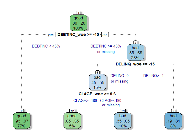
Well, this plot is beautiful looking and simple enough at the same time. The final decision tree model makes all predictions using just three features: debt-to-income ratio (DEBTINC), number of delinquent credit lines (DELINQ) and age of oldest credit line in months (CLAGE). For instance, if an applicant has a debt-to-income ratio above 45% and at least one delinquent credit line, the model flags him as a bad customer. The relative importance of the variables is shown in the next plot.
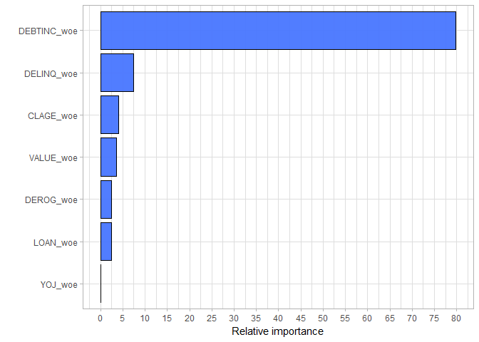
Obviously, DEBTINC is by far the strongest predictor in the model. We can also see that among the variables that did not enter the final model, the value of the current property (VALUE), number of major derogatory reports (DEROG) and amount of the loan (LOAN) are the most significant.
Indeed, we got a really simple and logical model, but what about its predictive power? To answer this question, we need to compute the model’s AUC.
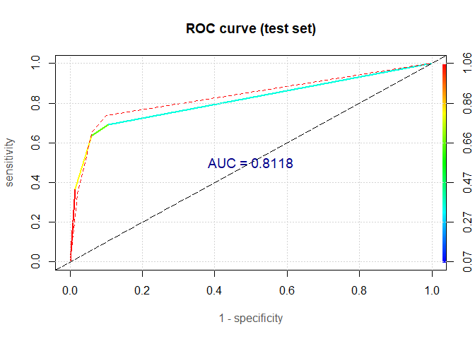
The red dashed line represents the ROC curve for the training sample, while multicolour full line represents the ROC curve for the test sample. Although the AUC on the test set is reasonably high ( 81.2%), it is considerably less than the AUC for the logistic regression model ( 90.1%). This is not surprising at all, and, in practice, decision trees are mostly used for variable selection or segmentation.
Ensemble Methods
The idea behind ensemble methods is to build numerous models and then combine their predictions to make a final prediction. It has been shown that in many cases ensemble methods outperform the simple models, such as logistic regression.
Decision trees are quite often used in ensemble methods. In this section, we will present two extremely popular ensemble methods: random forest and boosting.
Random Forest
“The steps for building a random forest are:
- Take a bootstrap sample
- Build a decision tree whereby for each node of the tree you randomly choose m inputs on which to base the splitting decision
- Split on the best of this subset
- Fully grow each tree without pruning”
B. Baesens, Analytics in a Big Data World, Wiley, 2014.
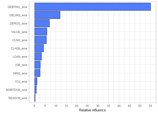
We are going to estimate our random forest model in R using randomForest() function from (yes, you’ve guessed it) randomForest package. We set the number of variables randomly chosen as candidates at each split (mtry) to 3 and number of trees to grow (ntree) to 400. The relative importance of the predictors in the model are listed below:
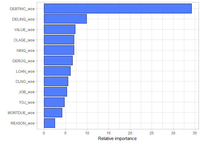
Once again, the variable DEBTINC is the best predictor. However, this time it is not as dominant as it was in the simple decision tree model. Furthermore, due to the randomness in the splitting process, all variables take a part in the random forest model. But did we improve the predictive performance?
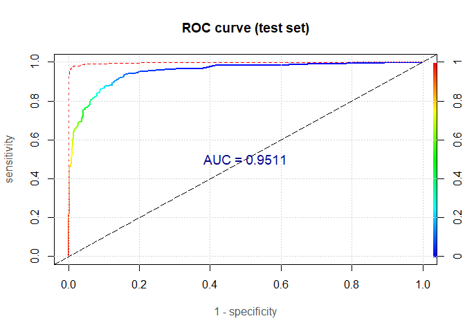
Yes, we did! We improved it a lot. We got the AUC on the test set of fantastic 95.1%! We now have a great predictive model. The only problem is that it is entirely a black box. We do not actually know how any particular variable is related to the model’s outcome. This could be irrelevant if you try, for instance, to detect a credit card fraud, but, in the credit scoring field, this is a highly undesirable characteristic. Thus, the logistic regression remains the go-to method.
Boosting
“Boosting works by estimating multiple models using a weighted sample of the data. Starting from uniform weights, boosting will iteratively reweight the data according to the classification error, whereby misclassified cases get higher weights.” (B. Baesens, Analytics in a Big Data World, Wiley, 2014)
To perform boosting in R you can use gbm() from the gbm package. Several parameters can affect the predictive performance of the boosted models. Thus, we had experimented a bit with parameters’ values before we chose our final model (train() from the caret package makes this task effortless). In the end, we set the total number of trees to fit ( n.trees) to 500, shrinkage parameter or learning rate ( shrinkage) to 0.2 and number of cross-validation folds to perform ( cv.folds) to 5.
The variable importance plot is telling us a similar story as in the random forest case.
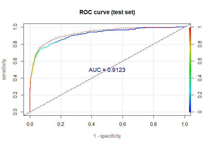
The AUC on the test set is 91.2%. This value is between the AUC for the logistic regression model and the AUC for the random forest model.
To conclude, we can certainly get somewhat better predictions by using ensemble methods, but if we are interested in building a credit risk scorecard, then we need to stick with our logistic regression model from Part Two.
Scorecard Development
A credit risk scorecard is just another way of presenting a linear model. The idea is to transform the estimated model’s coefficients into (more comprehensible) points.
We start with our logistic regression model:

where odds = P(bad) / P(good), WOEDEBTINC is the weight of evidence coded debt-to-income ratio, and so on.
We then express a score as a linear function of the ln(odds):

By combining last two equations we get:
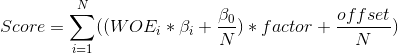
where N is the number of predictors.
We can easily compute offset and factor. Let’s say we want a score of 500 for odds of 1:1, and a score of 520 for odds of 1:2. This gives us the next two equations:
500 = offset + factor * ln( 1 / 1)
520 = offset + factor * ln( 1 / 2)
We then solve this system of equations and get that offset = 500 and factor = -28.85.
In R the scorecard() function carries out all this calculations and builds a scorecard. The results for some of the variables are presented in the following tables. The points assigned to each bin are displayed in the last column.
| bin | count | count\_distr | good | bad | badprob | woe | bin\_iv | total\_iv | points |
| \[-Inf,30) | 1,007 | 0.23 | 958 | 49 | 0.05 | -1.58 | 0.34 | 2.20 | 43 |
| \[30,45) | 2,445 | 0.55 | 2,262 | 183 | 0.07 | -1.13 | 0.48 | 2.20 | 30 |
| \[45, Inf) | 60 | 0.01 | 3 | 57 | 0.95 | 4.33 | 0.27 | 2.20 | -116 |
| missing | 959 | 0.21 | 356 | 603 | 0.63 | 1.92 | 1.10 | 2.20 | -51 |
| bin | count | count\_distr | good | bad | badprob | woe | bin\_iv | total\_iv | points |
| \[-Inf,1) | 3,122 | 0.70 | 2,672 | 450 | 0.14 | -0.39 | 0.09 | 0.68 | 11 |
| \[1,2) | 498 | 0.11 | 333 | 165 | 0.33 | 0.69 | 0.06 | 0.68 | -18 |
| \[2,3) | 184 | 0.04 | 105 | 79 | 0.43 | 1.10 | 0.07 | 0.68 | -30 |
| \[3,5) | 165 | 0.04 | 73 | 92 | 0.56 | 1.62 | 0.13 | 0.68 | -43 |
| \[5, Inf) | 61 | 0.01 | 3 | 58 | 0.95 | 4.35 | 0.28 | 0.68 | -117 |
| missing | 441 | 0.10 | 393 | 48 | 0.11 | -0.71 | 0.04 | 0.68 | 19 |
| bin | count | count\_distr | good | bad | badprob | woe | bin\_iv | total\_iv | points |
| \[-Inf,60) | 147 | 0.03 | 84 | 63 | 0.43 | 1.10 | 0.05 | 0.23 | -26 |
| \[60,120) | 1,051 | 0.24 | 769 | 282 | 0.27 | 0.39 | 0.04 | 0.23 | -9 |
| \[120,180) | 1,117 | 0.25 | 864 | 253 | 0.23 | 0.16 | 0.01 | 0.23 | -4 |
| \[180,240) | 1,000 | 0.22 | 851 | 149 | 0.15 | -0.35 | 0.02 | 0.23 | 8 |
| \[240, Inf) | 932 | 0.21 | 838 | 94 | 0.10 | -0.80 | 0.10 | 0.23 | 19 |
| missing | 224 | 0.05 | 173 | 51 | 0.23 | 0.17 | 0.001 | 0.23 | -4 |
We can now use this scorecard to score the applicants in our data set. This can be achieved with the function scorecard_ply().
| base\_points | YOJ\_points | CLNO\_points | JOB\_points | NINQ\_points | LOAN\_points | CLAGE\_points | VALUE\_points | DEROG\_points | DELINQ\_points | DEBTINC\_points | score |
| 520 | 1 | -12 | -6 | 0 | -27 | -9 | -14 | 4 | 11 | -51 | 417 |
| 520 | 1 | 5 | -6 | 2 | -27 | -4 | 3 | 4 | -30 | -51 | 417 |
| 520 | -6 | 5 | -6 | 0 | -27 | -4 | -32 | 4 | 11 | -51 | 414 |
| 520 | 13 | 0 | 33 | 5 | -27 | -4 | -107 | 15 | 19 | -51 | 416 |
| 520 | -6 | 5 | 15 | 2 | -27 | -9 | 8 | 4 | 11 | -51 | 472 |
| 520 | 1 | 5 | -6 | 0 | -27 | -9 | 3 | -55 | -30 | -51 | 351 |
Next, we can plot and compare the score distributions for the training and test set.
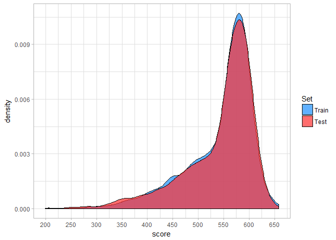
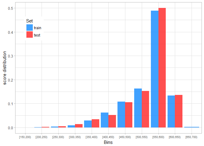
Clearly, the score distributions are rather close, so we can conclude that our scorecard makes reasonable predictions. This can also be confirmed by calculating a population stability index ( PSI). The PSI value of 0.01 indicates that actual distribution is almost the same as expected distribution.
End of Part Three
Well, this has been a long and wonderful journey, but as the old proverb says “All good things must come to an end”. The credit scoring walk-through is completed. It is finished and done! It is kaputt! It is no more! It has ceased to be! It has expired and gone to meet its maker! It is an ex-walk-through!