Credit Scoring Walk-through - Part Two
In Part One we demonstrated how to visually and statistically explore the data. In this post, we are going to apply the weight of evidence transformation to our predictors and then use logistic regression to develop our first credit scoring model.
Data Set: Home Equity Loans
The data set that was introduced in Part One will be also used here. Its characteristics are listed below:
- BAD: 1 = applicant defaulted on loan or seriously delinquent; 0 = applicant paid loan
- LOAN: Amount of the loan request
- MORTDUE: Amount due on existing mortgage
- VALUE: Value of current property
- REASON: DebtCon = debt consolidation; HomeImp = home improvement
- JOB: Occupational categories
- YOJ: Years at present job
- DEROG: Number of major derogatory reports
- DELINQ: Number of delinquent credit lines
- CLAGE: Age of oldest credit line in months
- NINQ: Number of recent credit inquiries
- CLNO: Number of credit lines
- DEBTINC: Debt-to-income ratio
Weight of Evidence Coding
The weight of evidence coding is basically a data pre-processing method. Its main idea is to replace the values of a continuous or categorical variable with the associated weight of evidence (WOE). This method allows us to keep missing values and outliers in the model development data set and enables us to include, if needed, non-linear relationships in a linear model.
The WOE is calculated using the formula:

Positive WOE means that, for the particular bin, the proportion of goods is larger than the proportion of bads.
Information Value (IV), on the other hand, measures the predictive power of a variable, and is defined by the equation:
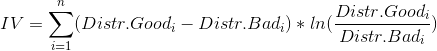
where n is the total number of bins. The relationship between IV and the variable’s predictive power is presented in the next table:
| IV | Predictive.power |
| below 0.02 | Useless for prediction |
| 0.02 to 0.10 | Weak predictor |
| 0.10 to 0.30 | Medium predictor |
| 0.30 to 0.50 | Strong predictor |
| above 0.50 | Suspicious or too good to be true |
There are many R packages that can be applied to calculate the weight of evidence and information value. Here, we will use quite versatile scorecard package. Its function woebin() performs automatic optimal binning for the predictors using tree-like segmentation, but it also offers you an option to pick your own breakpoints. However, it should be taken into account that woebin() computes WOE as ln(Distr.Badi / Distr.Goodi), so we need to multiply all resulting WOEs by -100 to get the values that are in line with our earlier definition.
For those who have her majesty R installed on their computer and are eager to experiment with WOE binning, you can use a simple Shiny application that I built specially for this occasion. You just need to run next two lines of code and off you go!
install.packages(c( "shiny", "ggplot2", "caret", "scorecard"))
shiny::runGitHub("woe_app", "carics")
But before we start, we have to say a few things. First, although we are going to compute and review many statistical measures, our main criterion for choosing the final binning is going to be the business logic. For instance, if we expect that variable’s attributes have a positive linear relationship with WOE, then every binning that does not satisfy this condition should be promptly rejected, no matter how high is the total information value. Second, to prevent overfitting, we set the minimum number of cases in a bin to 50. Finally, we will use solely training set to perform the binning.
And now, let us dive into the wonderful world of WOE binning.
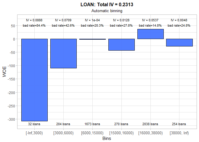
It is evident that smaller home equity loans are riskier than larger ones. This is something we have indeed expected. However, the data also show that at certain point loan’s risk stops decreasing and starts slowly increasing, although it never reaches the (high) risk level for the small loans. The manual binning is necessary due to the fact that first automatically selected bin has only 32 cases and that calculated intervals are not acceptable from the business point of view. For instance, is it reasonable to have a separate bin for loans that are between 15,000$ and 16,000$, such a narrow range? Surely, the answer is no. Thus, we decided to discard these bins and create the new ones that are equally spaced. Although IV dropped from 0.23 to 0.16 in the process, this is the price we should gladly pay to prevent overfitting and to get a meaningful scorecard in the end. Finally, it should be noted that reversal in the risk trend is incorporated at the loan amount of 30,000$.
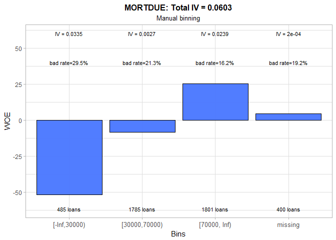
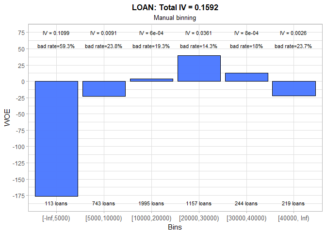
Automatic binning for the amount due on existing mortgage produces pretty messy bins: two of them have less than 50 observations and there is no visible trend in risk level. Even though overall IV is reasonably high (0.11), its value is not, under this circumstances, a good indicator of the characteristics’ predictive power. We decided to create three large groups (beside missing bin) and to introduce the positive linear relationship between MORTDUE and WOE values. As a consequence, IV fell to 0.06, but, at the same time, we got more justifiable bins.
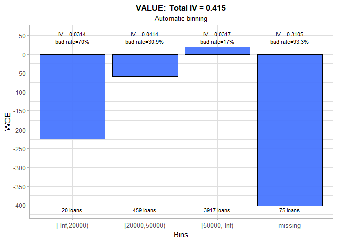
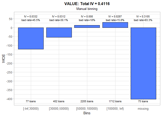
The only problem with automatic binning for VALUE is that the first bin consists of just 20 loans. Therefore, we set a higher upper limit for this bin. The linear trend is preserved and total IV practically remains unchanged.
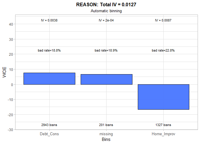
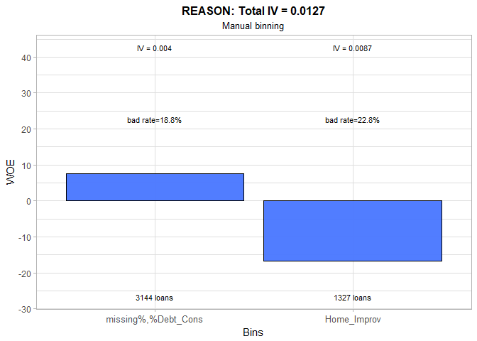
We merged missing and Debt Consumption categories because they have almost the identical bad rates. Nonetheless, the change we made is cosmetic. As we saw in Part One, the reason for a loan is not related to the obligors’ creditworthiness and IV of 0.01 fully supports this conclusion.
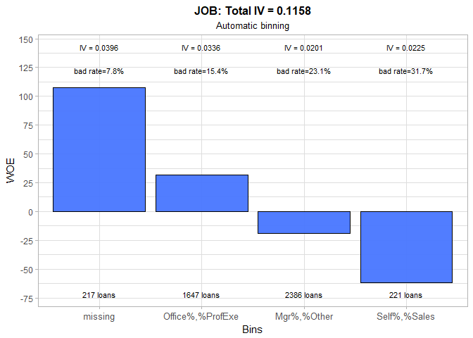
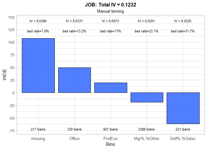
The JOB variable seems to be moderately predictive. In comparison to automatic binning, we chose to keep Office and Professional Executive categories separated, and as a result achieve a small increase in variable’s IV. However, it is surprising that customers with unknown (e.g. missing) occupation are the least risky ones. If we cannot find a rational reason behind this, we could decide to set the WOE value for the missing group to zero. By doing so, we will not award our future applicants for hiding their occupation information from us. And in case we are deeply pessimistic about human nature, we could even assign them some negative WOE value or treat them like they belong to the riskiest group.
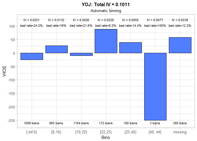
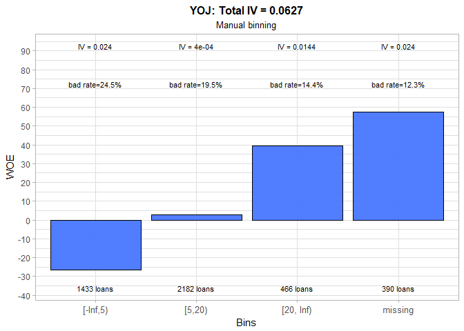
The business experience shows that people who work longer at their current job are more likely to repay a debt. Hence, we immediately dismissed the outcome of automatic binning and proceeded to manual binning. Three large groups are formed and a positive trend in WOE values is established. Unfortunately, total IV significantly decreased in the process. Once again, the missing category has the lowest bad rate. All previously mentioned solutions to this problem are at our disposal.
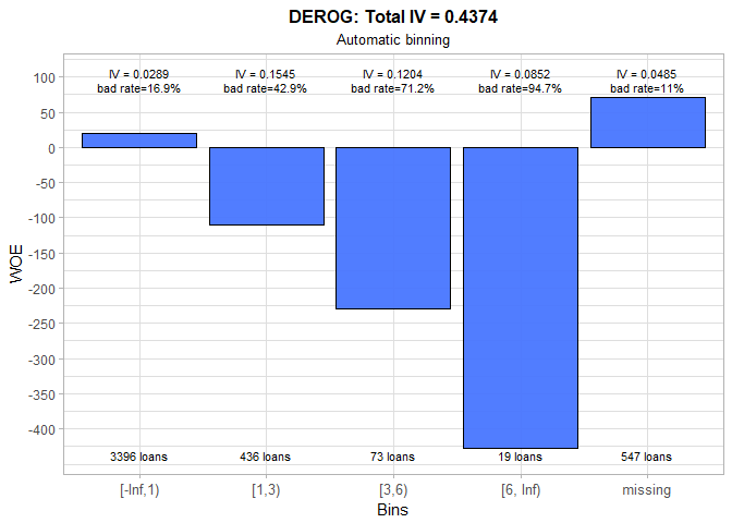
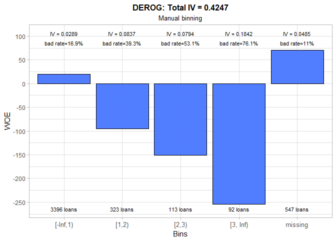
The trend in WOE for the number of major derogatory reports is negative and this is something we expected to see. We keep the number of groups that were chosen by automatic binning, but we make few changes in the cut-offs. Consequently, total IV only marginally decreased.
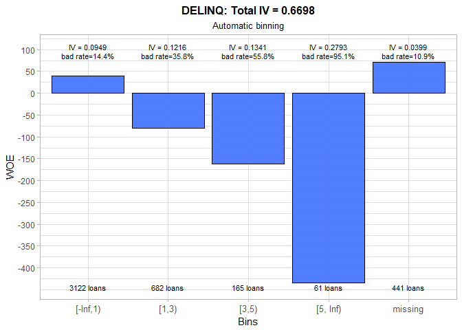
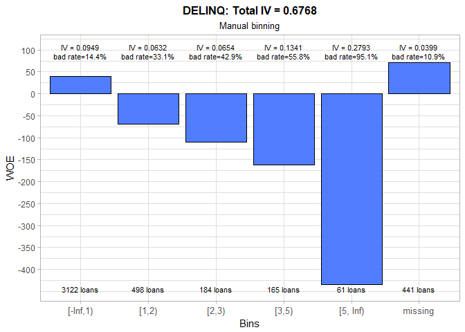
The number of delinquent credit lines is obviously a strong predictor of someone’s credit performance. For example, the person with 5 or more delinquent credit lines will almost certainly default on the loan. The strange occurrence is a below average bad rate for the missing group and it should definitely be inspected.
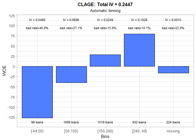
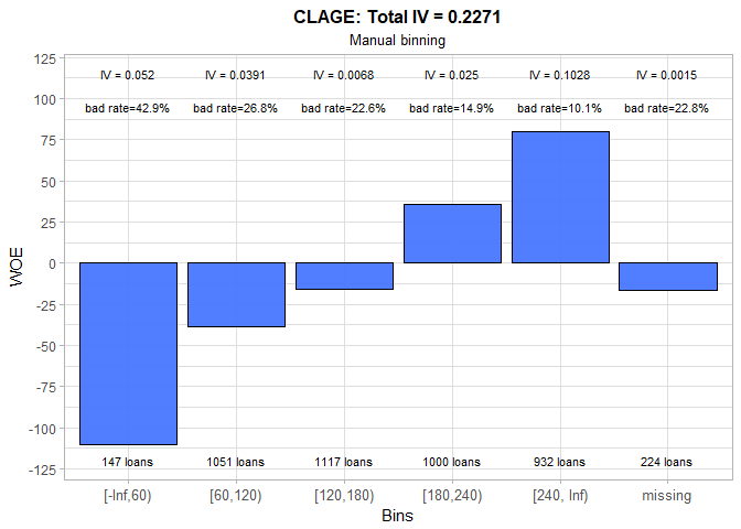
Although automatic binning produces a sound result for the CLAGE variable, we modified constructed bins to incorporate business logic. Therefore, we picked our cutoffs to be the exact number of years (e.g. 60 months = 5 years, 240 months = 20 years). The WOE values exhibit a clear positive trend, and it appears that missing group is most similar to the middle group (120-180 months). Based on its IV, this variable is a medium predictor.
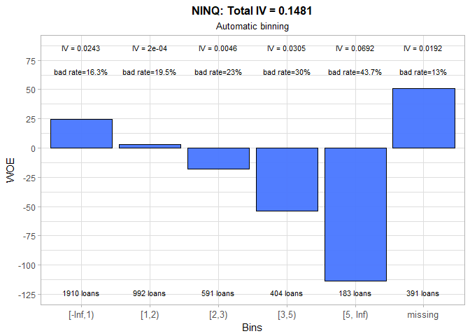
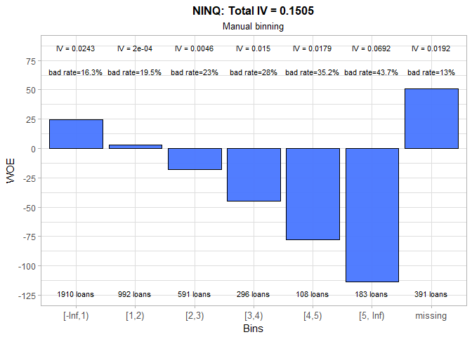
As expected, the higher the number of recent credit inquiries, the higher the chance that obligor will default. We made a small adjustment to initially calculated bins, thereby slightly increasing the total IV. The one more time, missing category has a suspiciously low bad rate.
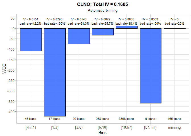
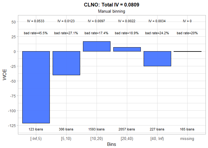
For the number of credit lines, the automatic binning produced quite confusing results, so we manually set more business-like intervals. Although IV halved, new bins better capture non-linearities in the data. The riskiest are the applicants with less than 5 credit lines, while the most creditworthy are those who have between 10 and 20 credit lines.
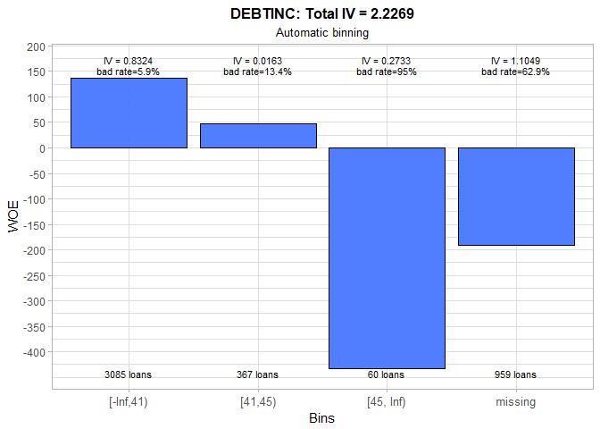
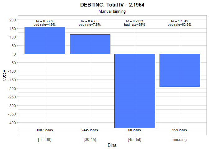
The huge IV value of 2.19 for DEBTINC reveals that this variable is an extremely strong predictor of someone’s probability of default. A debt-to-income ratio that is over 45% is a firm indicator of the future debt repayment issues and, thus, could be used as one of the policy rules for instantaneously declining potential customers. In addition, the people with non-available debt-to-income ratio are, as expected, much riskier than an average applicant.
The manual binning is finally done and, after all this tedious diligent work, we can rank our predictors by their information value:
| Variable | IV |
| DEBTINC | 2.195 |
| DELINQ | 0.677 |
| DEROG | 0.425 |
| VALUE | 0.412 |
| CLAGE | 0.227 |
| LOAN | 0.159 |
| NINQ | 0.151 |
| JOB | 0.123 |
| CLNO | 0.081 |
| YOJ | 0.063 |
| MORTDUE | 0.060 |
| REASON | 0.013 |
We are now able to convert our training and test set (which were created in Part One) to the weight of evidence values. We are going to use the function woebin_ply() for this purpose.
| REASON\_woe | MORTDUE\_woe | YOJ\_woe | CLNO\_woe | JOB\_woe | NINQ\_woe | LOAN\_woe | CLAGE\_woe | VALUE\_woe | DEROG\_woe | DELINQ\_woe | DEBTINC\_woe | BAD |
| 0.1674 | 0.5174 | -0.0270 | 0.4010 | 0.1887 | -0.0313 | 1.7654 | 0.3862 | 0.5468 | -0.2011 | -0.3920 | 1.9164 | bad |
| 0.1674 | -0.2531 | -0.0270 | -0.1690 | 0.1887 | -0.2480 | 1.7654 | 0.1612 | -0.1297 | -0.2011 | 1.1049 | 1.9164 | bad |
| 0.1674 | 0.5174 | 0.2636 | -0.1690 | 0.1887 | -0.0313 | 1.7654 | 0.1612 | 1.2071 | -0.2011 | -0.3920 | 1.9164 | bad |
| -0.0759 | -0.0445 | -0.5742 | 0.0031 | -1.0757 | -0.5077 | 1.7654 | 0.1679 | 4.0284 | -0.7045 | -0.7132 | 1.9164 | bad |
| 0.1674 | -0.2531 | 0.2636 | -0.1690 | -0.4945 | -0.2480 | 1.7654 | 0.3862 | -0.2860 | -0.2011 | -0.3920 | 1.9164 | good |
| 0.1674 | 0.0818 | -0.0270 | -0.1690 | 0.1887 | -0.0313 | 1.7654 | 0.3862 | -0.1297 | 2.5468 | 1.1049 | 1.9164 | bad |
Logistic Regression Model
At last, the time has come for us to create our first credit scoring model. We will apply logistic regression (glm() in R), which is hands down the most popular statistical method for building this type of models. Furthermore, a stepwise algorithm (step()) will be employed to eliminate non-predictive variables from the initial model that uses all possible characteristics. The outcome is shown in the following table:
| BAD | |
| YOJ\_woe | -0.008\*\*\* |
| (-0.002) | |
| CLNO\_woe | -0.010\*\*\* |
| (-0.002) | |
| JOB\_woe | -0.010\*\*\* |
| (-0.002) | |
| NINQ\_woe | -0.003\*\* |
| (-0.001) | |
| LOAN\_woe | -0.005\*\*\* |
| (-0.001) | |
| CLAGE\_woe | -0.008\*\*\* |
| (-0.001) | |
| VALUE\_woe | -0.009\*\*\* |
| (-0.001) | |
| DEROG\_woe | -0.007\*\*\* |
| (-0.001) | |
| DELINQ\_woe | -0.009\*\*\* |
| (-0.001) | |
| DEBTINC\_woe | -0.009\*\*\* |
| (-0.000) | |
| Constant | 0.014\*\*\* |
| (-0.001) | |
| Observations | 4,471 |
| Log Likelihood | -1,155.082 |
| Akaike Inf. Crit. | 2,332.164 |
| Notes: | \*\*\*Significant at the 1 percent level. |
| \*\*Significant at the 5 percent level. | |
| \*Significant at the 10 percent level. | |
As we can see, variables REASON and MORTDUE are excluded from the final model. The remaining variables are statistically significant at the 0.05 level, and their coefficients have the expected sign (i.e. the WOE values are negatively related to the probability of default).
To evaluate the performance of our credit scoring model, we can use many statistical measures. The most well-known is the area under the ROC curve (AUC). It represents the probability that a randomly chosen bad loan will have a higher probability of default than a randomly chosen good loan. Some other useful measures are accuracy, sensitivity, specificity, Gini coefficient and Kolmogorov-Smirnov (KS) statistic.
AUC benchmarks for various analytics applications are illustrated in the table:
| Application | Number.of.Characteristics | AUC.Ranges |
| Application credit scoring | 10-15 | 0.70-0.85 |
| Behavioral credit scoring | 10-15 | 0.80-0.90 |
| Churn detection (telco) | 6-10 | 0.70-0.90 |
| Fraud detection (insurance) | 10-15 | 0.70-0.90 |
source: Bart Baesens, Analytics in a Big Data World, Wiley, 2014.
We now use the logistic regression model to predict probabilities of default on the training and test set. These are then used to generate the ROC curve and compute AUC, Gini and KS statistic.
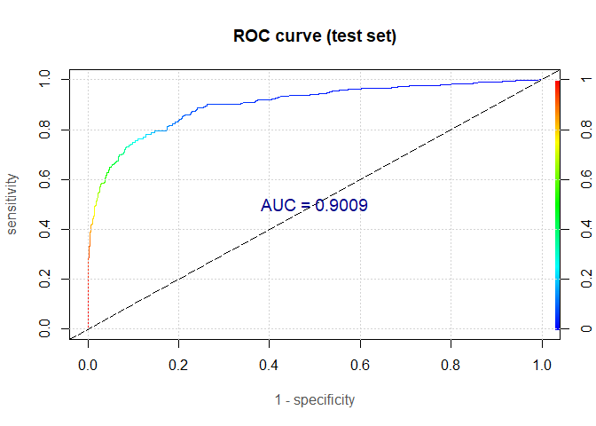
| Measure | Training.set | Test.set |
| AUC | 0.919 | 0.900 |
| Gini | 0.675 | 0.637 |
| KS | 0.693 | 0.643 |
The computed measures are somewhat lower on the test set, so there is a small amount of overfitting. That being said, we got the AUC value of outstanding 90.1%. The model is without a doubt doing a great job in discriminating the good loans from the bad ones.
End of Part Two
WOE, IV, KS, AUC… Are we once and for all done with these hellish acronyms? Sadly, just for the day. In Part Three we will show some alternative methods that can be employed to estimate the credit scoring models. Nevertheless, the current logistic regression model will remain “the chosen one” and will be used in the second half of the next post for building a credit risk scorecard.