Credit Scoring Walk-through - Part One
A credit scoring model is a statistical tool widely used by lenders to assess the creditworthiness of their potential and existing customers. The basic idea behind this model is that various demographic attributes and past repayment behaviour of an individual can be utilized to predict hers or his probability of default.
This blog post will mostly cover the first phase of every model development project: data exploration and preparation.
Data Set: Home Equity Loans
For demonstration purposes, we will be using the data set that contains characteristics and delinquency information for 5,960 home equity loans (source: B. Baesens, D. Roesch, H. Scheule, Credit Risk Analytics: Measurement Techniques, Applications and Examples in SAS, Wiley, 2016). The data set variables are:
- BAD: 1 = applicant defaulted on loan or seriously delinquent; 0 = applicant paid loan
- LOAN: Amount of the loan request
- MORTDUE: Amount due on existing mortgage
- VALUE: Value of current property
- REASON: DebtCon = debt consolidation; HomeImp = home improvement
- JOB: Occupational categories
- YOJ: Years at present job
- DEROG: Number of major derogatory reports
- DELINQ: Number of delinquent credit lines
- CLAGE: Age of oldest credit line in months
- NINQ: Number of recent credit inquiries
- CLNO: Number of credit lines
- DEBTINC: Debt-to-income ratio
The binary variable BAD will be the target variable in our credit scoring model, while other variables will be used as predictors. The first six observations (i.e. loans) of the data set are given below:
| BAD | LOAN | MORTDUE | VALUE | REASON | JOB | YOJ | DEROG | DELINQ | CLAGE | NINQ | CLNO | DEBTINC | BADn |
| bad | 1,100 | 25,860 | 39,025 | HomeImp | Other | 10.5 | 0 | 0 | 94.4 | 1 | 9 | 1 | |
| bad | 1,300 | 70,053 | 68,400 | HomeImp | Other | 7 | 0 | 2 | 121.8 | 0 | 14 | 1 | |
| bad | 1,500 | 13,500 | 16,700 | HomeImp | Other | 4 | 0 | 0 | 149.5 | 1 | 10 | 1 | |
| bad | 1,500 | 1 | |||||||||||
| good | 1,700 | 97,800 | 112,000 | HomeImp | Office | 3 | 0 | 0 | 93.3 | 0 | 14 | 0 | |
| bad | 1,700 | 30,548 | 40,320 | HomeImp | Other | 9 | 0 | 0 | 101.5 | 1 | 8 | 37.1 | 1 |
Next, we will take a look at some basic summary statistics for our variables:
##    BAD            LOAN          MORTDUE           VALUE
##  good:4771   Min.   : 1100   Min.   :  2063   Min.   :  8000
##  bad :1189   1st Qu.:11100   1st Qu.: 46276   1st Qu.: 66076
##              Median :16300   Median : 65019   Median : 89236
##              Mean   :18608   Mean   : 73761   Mean   :101776
##              3rd Qu.:23300   3rd Qu.: 91488   3rd Qu.:119824
##              Max.   :89900   Max.   :399550   Max.   :855909
##                              NA's   :518      NA's   :112
##      REASON          JOB            YOJ             DEROG
##         : 252          : 279   Min.   : 0.000   Min.   : 0.0000
##  DebtCon:3928   Mgr    : 767   1st Qu.: 3.000   1st Qu.: 0.0000
##  HomeImp:1780   Office : 948   Median : 7.000   Median : 0.0000
##                 Other  :2388   Mean   : 8.922   Mean   : 0.2546
##                 ProfExe:1276   3rd Qu.:13.000   3rd Qu.: 0.0000
##                 Sales  : 109   Max.   :41.000   Max.   :10.0000
##                 Self   : 193   NA's   :515      NA's   :708
##      DELINQ            CLAGE             NINQ             CLNO
##  Min.   : 0.0000   Min.   :   0.0   Min.   : 0.000   Min.   : 0.0
##  1st Qu.: 0.0000   1st Qu.: 115.1   1st Qu.: 0.000   1st Qu.:15.0
##  Median : 0.0000   Median : 173.5   Median : 1.000   Median :20.0
##  Mean   : 0.4494   Mean   : 179.8   Mean   : 1.186   Mean   :21.3
##  3rd Qu.: 0.0000   3rd Qu.: 231.6   3rd Qu.: 2.000   3rd Qu.:26.0
##  Max.   :15.0000   Max.   :1168.2   Max.   :17.000   Max.   :71.0
##  NA's   :580       NA's   :308      NA's   :510      NA's   :222
##     DEBTINC              BADn
##  Min.   :  0.5245   Min.   :0.0000
##  1st Qu.: 29.1400   1st Qu.:0.0000
##  Median : 34.8183   Median :0.0000
##  Mean   : 33.7799   Mean   :0.1995
##  3rd Qu.: 39.0031   3rd Qu.:0.0000
##  Max.   :203.3121   Max.   :1.0000
##  NA's   :1267
As we can see, there is a decent amount of missing values (NA’s). So, what should we do? The easiest approach, obviously, is to delete all the observations that contain them (e.g. na.omit() in R would do the trick) and then act like they have never existed. But if we actually decided to do this, we would loose almost two-fifths of our initial data set! Another option is to impute (i.e. replace) the missing values with some logical values. For example, we could use the mean or median to replace NA values for the continuous variables, or mode for the categorical ones. Or we could apply more complex imputation methods, such as multivariate imputation by chained equations (in R the mice package implements this method). Unfortunately, in most cases imputation methods, even the most sophisticated ones (that sip Merlot while reading Walt Whitman poems next to the fireplace), add little, if anything, to the model’s performance. Lastly, the third approach is to keep the missing values in the data set, as they can actually be quite informative. For instance, if someone’s income is missing, the explanation could be that he or she is currently unemployed. If missing values are related to the target variable, then the best course of action is to keep them in the model development data set (we will see in Part Two how this can be stylishly achieved with Weight of evidence coding).
But before we deal with our precious missing data, we should fully direct attention to non-missing data. After all, models are all about non-missing data (No offense, dear NA’s). Thus, let us now draw some nice-looking (gg)plots.
Data Exploration
The first variable we analyse is BAD, which will be the target variable in our credit scoring model.
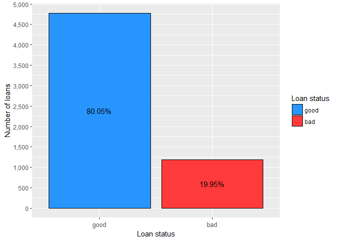
This simple bar plot shows that the proportion of bad applicants (those who are seriously delinquent or already defaulted) in the data set is about 20%. The total number of ‘bads’ (roughly 1,200) is more or less acceptable for the model development.
“Typically about a minimum of 2,000 each of goods, bads, and rejects are sufficient for scorecard development.” (N. Siddiqi, Intelligent Credit Scoring: Building and Implementing Better Credit Risk Scorecards, Wiley, 2017)
Our next step is to visually inspect the relationship between the target variable and other variables in the data set. For the categorical variables and continuous variables with relatively small number of possible values we will use bar plots. On the other hand, for the “regular” continuous variables we will produce their density curves.
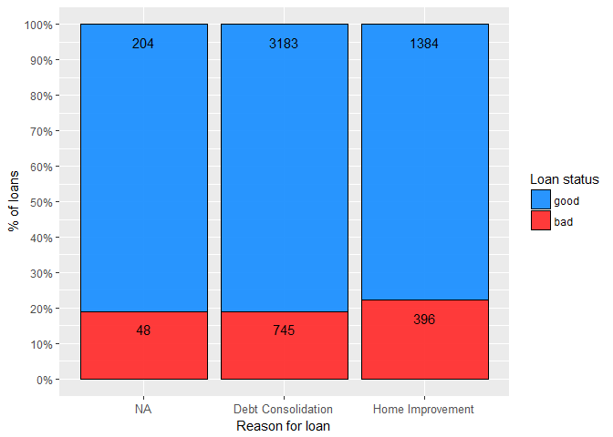
It is obvious that the bad rate ( bads/(goods+bads) ) is roughly the same no matter what is the reason for a loan. In fact, calculated Cramer’s V value (CramerV() from DescTools was used) of just 0.04 confirms this conclusion, with 0.10 commonly used in industry as a cutoff value. Furthermore, it seems that missing values, in this case, care no valuable information.
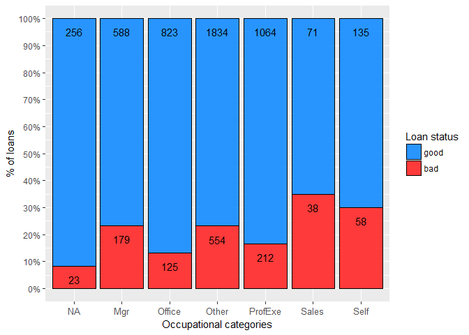
Clearly, the occupation of the applicant matters (Cramer’s V = 0.13). For instance, the bad rate for a salesperson is almost three times as high as for an office worker. Also, in this data set the lowest risk, surprisingly, exhibit the obligors whose occupation information is not available.
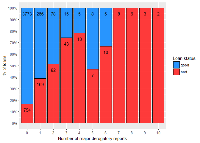
As expected, the higher the number of major derogatory reports, the greater the risk. This variable is continuous, but it could be easily, and probably without much loss of information, converted to ordinal factor variable (e.g. zero, one, and two or more reports).
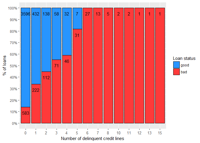
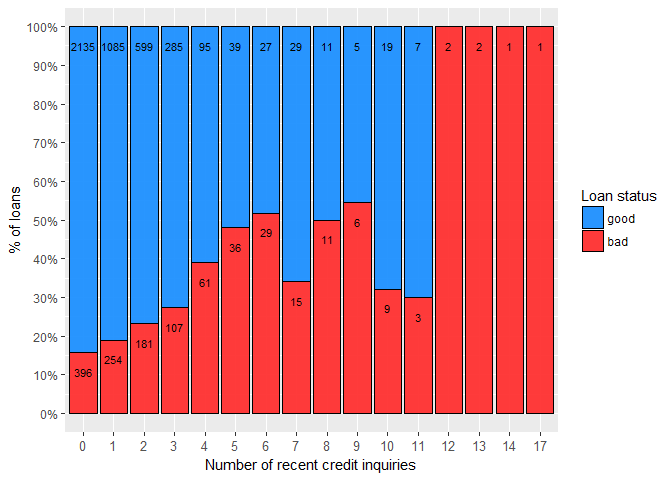
The variables DELINQ and NINQ exhibit similar behaviour as previously mentioned DEROG variable, so they too can be transformed into discrete variables.
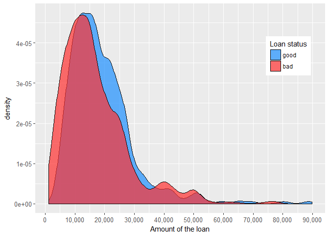
It seems that the applicants who took smaller home equity loans are somewhat riskier than those with larger ones. One possible explanation could be that application process for the higher loans is more rigorous.
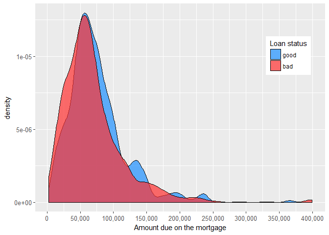
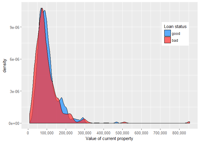
At first glance, the amount due on the mortgage and value of current property don’t seem to be especially related to the likelihood that applicant will repay a debt.
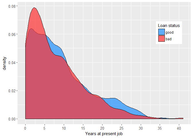
On the other hand, people who don’t change their jobs so often seem to be safer bet for the lender.
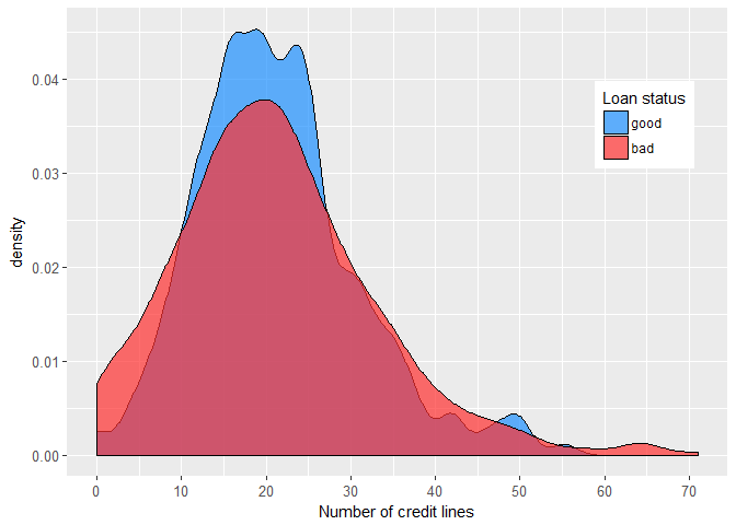
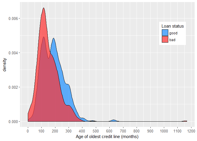
Further, it appears that the number of credit lines and age of the oldest credit line are to some extent related to the individual’s credit risk.
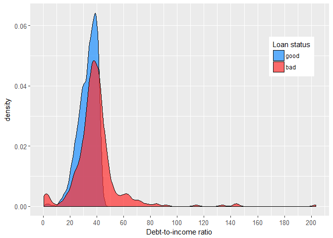
Finally, debt-to-income ratio is definitely positively associated with the probability of default on home equity loan.
In addition, we can run some statistical test to evaluate the predictive power of the discussed continuous variables. Individual t-test results are shown in the following table:
| variable | t.stat | p.value |
| LOAN | 5.72 | 0 |
| MORTDUE | 3.38 | 0.001 |
| VALUE | 1.86 | 0.06 |
| YOJ | 4.66 | 0.000003 |
| DEROG | -12.76 | 0 |
| DELINQ | -17.01 | 0 |
| CLAGE | 12.96 | 0 |
| NINQ | -10.53 | 0 |
| CLNO | 0.28 | 0.78 |
| DEBTINC | -6.90 | 0 |
Well, that’s all great, but what about those missing values? They are not present in any of displayed visual and statistical analysis. T-test just doesn’t give a damn about them, but we should. Hence, for each continuous variable we calculate the bad rate for missing data and compare it with the bad rate for available data.
| variable | bad.rate.non.missing | bad.rate.missing |
| LOAN | 19.95 | NA |
| MORTDUE | 19.9 | 20.46 |
| VALUE | 18.54 | 93.75 |
| YOJ | 20.64 | 12.62 |
| DEROG | 20.98 | 12.29 |
| DELINQ | 20.76 | 12.41 |
| CLAGE | 19.66 | 25.32 |
| NINQ | 20.44 | 14.71 |
| CLNO | 19.8 | 23.87 |
| DEBTINC | 8.59 | 62.04 |
The most notable differences in bad rates are present for the value of current property (VALUE) and debt-to-income ratio (DEBTINC). The missing data bad rate for VALUE is striking 94%, although it is obtained for only 112 loans, or less than 2% of the data set. On the other hand, this bad rate is 62% for DEBTINC, but it is attributed to more than one-fifth of all loans. All things considered, the missing values should certainly be kept in the data set.
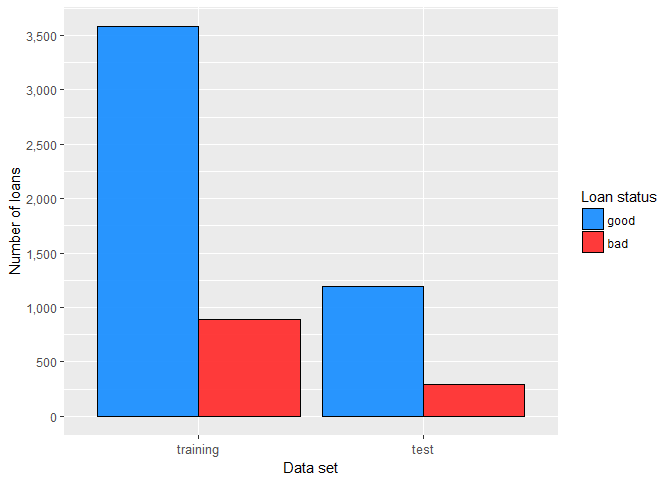
Training and Test Set
Before proceeding to model development, it is necessary to divide our data set into training and test set. Model(s) will be then developed using exclusively the training sample, while the test sample will be used for model validation. In our case, training sample will contain three-quarters of the data set and it will be stratified by target variable, therefore bad rate will be the same for both samples (in R this can be accomplished with createDataPartition() function from caret package). The final partition is shown in the bar plot.
End of Part One
So far we have thoroughly explored the data set, gained insights into its characteristics and possible caveats, visually and statistically examined associations of our soon-to-be predictors with the target variable, and created training and test sample, which will be used in model development and validation process. In Part Two we are going to introduce weight of evidence coding, apply it to the independent variables and build our first credit scoring model.